Brain Perfusion Analysis

What it does

Computes perfusion maps (CBF, CBV, MTT, Tmax) from a 4D CT or MR acquisition; in stroke mode it estimates the ischaemic core/penumbra mismatch, in tumour mode it highlights hyperperfused regions.

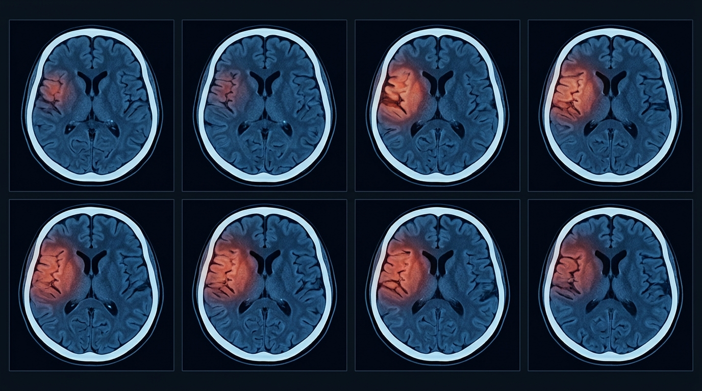
What perfusion is, and why it is done

A perfusion study measures physiology rather than anatomy: not how tissue looks, but how much blood passes through it. A bolus of contrast is injected and the same slices are scanned dozens of times over while it passes. What is analysed is not any single image but the intensity-against-time curve in every voxel — how quickly contrast arrives, how high it peaks, how fast it washes out.

In stroke this answers what a plain CT cannot answer in the first hours, while the infarct is still invisible: how much brain is already dead, and how much is alive but starving. The dead part — the core — will not recover. The starving part — the penumbra — is being held by collateral flow and can recover if perfusion is restored. The size of one against the other is what says whether reperfusion still has anything to save, and it is why perfusion is done urgently.

In a tumour the question is how much new vasculature it has built. Grade correlates with neoangiogenesis: a tumour that is actively growing perfuses more than the tissue around it. That shows in relative blood volume where ordinary contrast enhancement does not separate active tumour from post-treatment change.

The study. A perfusion series — the same slices scanned repeatedly while the bolus passes. CT and MR both work; the modality is read from the DICOM tag, and on MR the signal is converted to ΔR2* using the echo time. Five time frames is the minimum; below that the analysis does not run. The 4D volume is rebuilt from the slice and timing tags, so a series stripped of them may come back mis-ordered.

Optional. Contrast volume, patient weight and iodine concentration. They are used for the iodine-per-kg check only and change nothing in the maps.

How it is computed, and how to read it

From signal to concentration. On CT the rise in attenuation is proportional to iodine concentration, so the curve in Hounsfield units is already the concentration curve. On MR the signal drops instead, and is converted to ΔR2* = −ln(S/S₀)/TE.

The arterial input. To know what the tissue received, the concentration curve in a large artery is needed. It is found automatically: candidate voxels whose curve has the wrong shape — a late peak, too broad, a drifting baseline — are rejected, the rest are clustered by shape, and the median of the winning cluster becomes the input function. It is shown with a confidence figure and the voxel it was taken from.

Deconvolution. A tissue curve is the arterial input smeared out by the passage through the capillary bed. Undoing that smearing gives the residue function: its maximum is CBF, and the moment it peaks is Tmax. The method used here is block-circulant SVD. Ordinary SVD is sensitive to a late-arriving bolus — it overestimates Tmax and underestimates CBF precisely where blood arrives late, in stenosis and collateral flow, which is where the measurement matters most. The block-circulant form makes the result insensitive to that delay.

Volume and transit time. CBV is the area under the tissue curve divided by the area under the input curve; MTT follows from the central volume theorem as CBV/CBF.

Calibration. An input sampled from a small artery is underestimated by partial-volume averaging, which pushes CBF and CBV up. A venous curve from a large sinus, where that error is negligible, is found as well, and the maps are scaled by the ratio of the two areas. Relative CBV is additionally referenced to normal white matter, because absolute values depend on technique.

How to read it

Normal values, and what a deviation means:

Parameter	Normal	What a deviation means
CBF	20–80 mL/100g/min	Reduced — hypoperfusion. How far it is reduced is what separates core from penumbra.
CBV	2–5 mL/100g	Preserved or raised in penumbra — autoregulation is compensating. Reduced in the core.
MTT	4–6 s	Prolonged — slowed or collateral flow.
Tmax	< 6 s	Above 6 s — hypoperfused tissue at risk.
rCBV	≈ 1	Above 1.75 — the conventional high-grade pattern.

Stroke mode computes CBF, CBV, MTT and Tmax; tumour mode computes CBF, CBV, rCBV and PS.

Stroke. Reduced CBF with preserved CBV is penumbra — autoregulation has dilated the vessels and is holding the tissue. Reduced CBF with reduced CBV is core, where autoregulation is exhausted. Tissue past the 6 s Tmax threshold is the hypoperfused volume, and it is the mismatch between that and the core that says whether reperfusion has anything to save.

Tumour. rCBV above 1.75 is the conventional high-grade cut-off. PS reflects breakdown of the blood-brain barrier and rises in malignancy and in active inflammation alike, so it is read together with rCBV rather than on its own.

Check the input curve before trusting an absolute number. Every absolute value is scaled by that one curve. If its confidence is low, or the quality-control plot does not show a sharp early peak, read the maps by asymmetry against the opposite hemisphere rather than by the figures.

What the module takes on

It locates the arterial input, reports how confident that detection is and shows a warning when the confidence is low. It locates the venous curve and applies the partial-volume calibration. It draws the quality-control plot so the input can be checked by eye against the tissue curves. It measures the share of brain past each threshold — Tmax over 6 s, rCBV over 1.75 — and states the resulting pattern in one line. The maps, the curves and a PDF report are attached back to the study in PACS.

Wu O, Østergaard L, Weisskoff RM, Benner T, Rosen BR, Sorensen AG. “Tracer arrival timing-insensitive technique for estimating flow in MR perfusion-weighted imaging using singular value decomposition with a block-circulant deconvolution matrix.” Magn Reson Med. 2003;50(1):164–174. Partial-volume correction after Calamante F. (2007), Sourbron S. (2013).